── Attaching core tidyverse packages ──────────────────────── tidyverse 2.0.0 ──
✔ dplyr     1.1.4     ✔ readr     2.1.5
✔ forcats   1.0.0     ✔ stringr   1.5.1
✔ ggplot2   3.5.1     ✔ tibble    3.2.1
✔ lubridate 1.9.3     ✔ tidyr     1.3.1
✔ purrr     1.0.2
── Conflicts ────────────────────────────────────────── tidyverse_conflicts() ──
✖ dplyr::filter() masks stats::filter()
✖ dplyr::lag()    masks stats::lag()
ℹ Use the conflicted package (<http://conflicted.r-lib.org/>) to force all conflicts to become errors
library(maps)
Warning: package 'maps' was built under R version 4.4.2
Attaching package: 'maps'

The following object is masked from 'package:purrr':

    map
library(usmap)
Warning: package 'usmap' was built under R version 4.4.2
library(plotly)
Attaching package: 'plotly'

The following object is masked from 'package:ggplot2':

    last_plot

The following object is masked from 'package:stats':

    filter

The following object is masked from 'package:graphics':

    layout
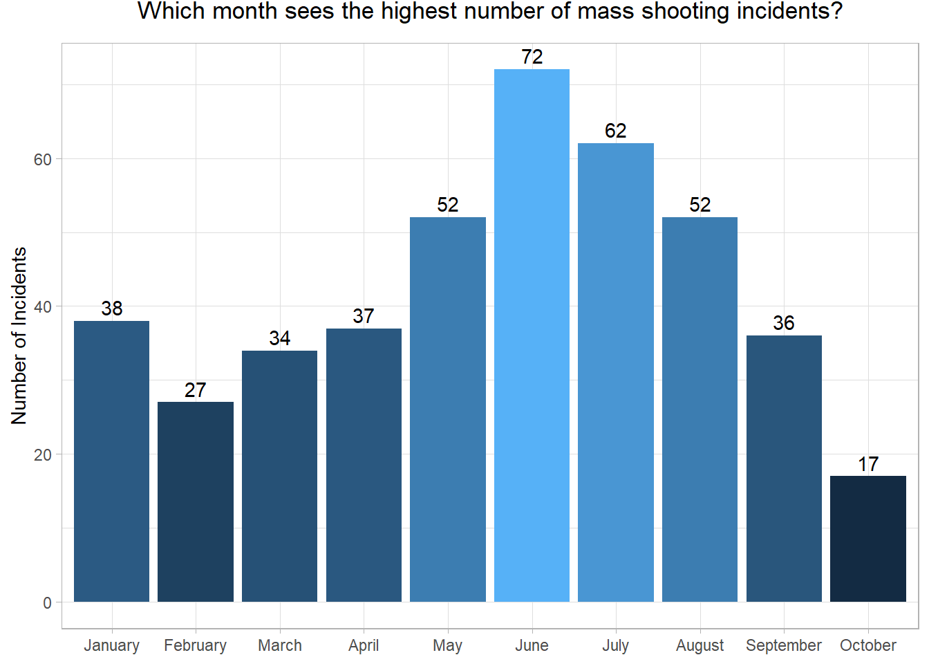
df_time |>group_by(month)|>summarize(month_count =n())|>ggplot(aes(x = month, y = month_count, fill = month_count))+geom_col()+geom_text(aes(label = month_count), vjust =-0.4) +labs(title ="Which month sees the highest number of mass shooting incidents?",x =NULL,y ="Number of Incidents" ,legend =NULL)+theme_light()+theme(plot.title =element_text(hjust=.5, vjust =3))+theme(legend.position ="none")
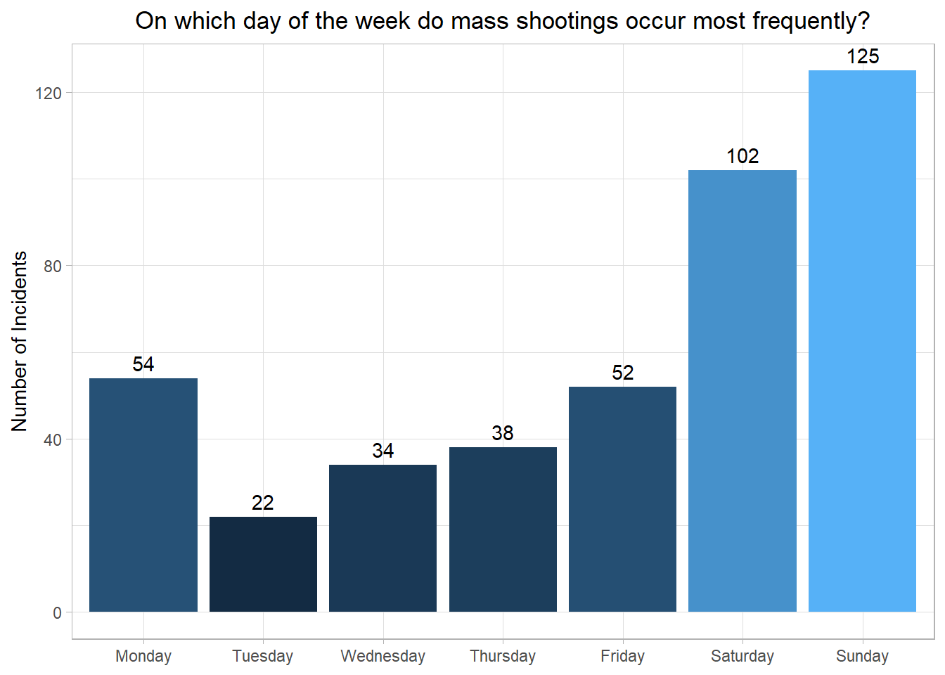
df_time |>group_by(en_weekday)|>summarize(day_count=n())|>ggplot(aes(x = en_weekday, y = day_count, fill = day_count))+geom_col()+geom_text(aes(label = day_count), vjust =-0.5) +labs(title ="On which day of the week do mass shootings occur most frequently?",x =NULL,y ="Number of Incidents" )+theme_light()+theme(plot.title =element_text(hjust=0.5))+theme(legend.position ="none")
# A tibble: 188 × 2
   date            date_sum
   <chr>              <int>
 1 March 31, 2024         9
 2 July 28, 2024          8
 3 July 4, 2024           8
 4 July 5, 2024           8
 5 June 23, 2024          8
 6 May 18, 2024           7
 7 August 25, 2024        6
 8 August 4, 2024         6
 9 June 15, 2024          6
10 June 2, 2024           6
# ℹ 178 more rows
# A tibble: 188 × 2
   date               cas_sum
   <chr>                <dbl>
 1 June 2, 2024            59
 2 July 4, 2024            56
 3 June 23, 2024           47
 4 June 15, 2024           45
 5 September 21, 2024      43
 6 July 5, 2024            42
 7 March 31, 2024          42
 8 July 28, 2024           39
 9 May 18, 2024            39
10 October 12, 2024        38
# ℹ 178 more rows
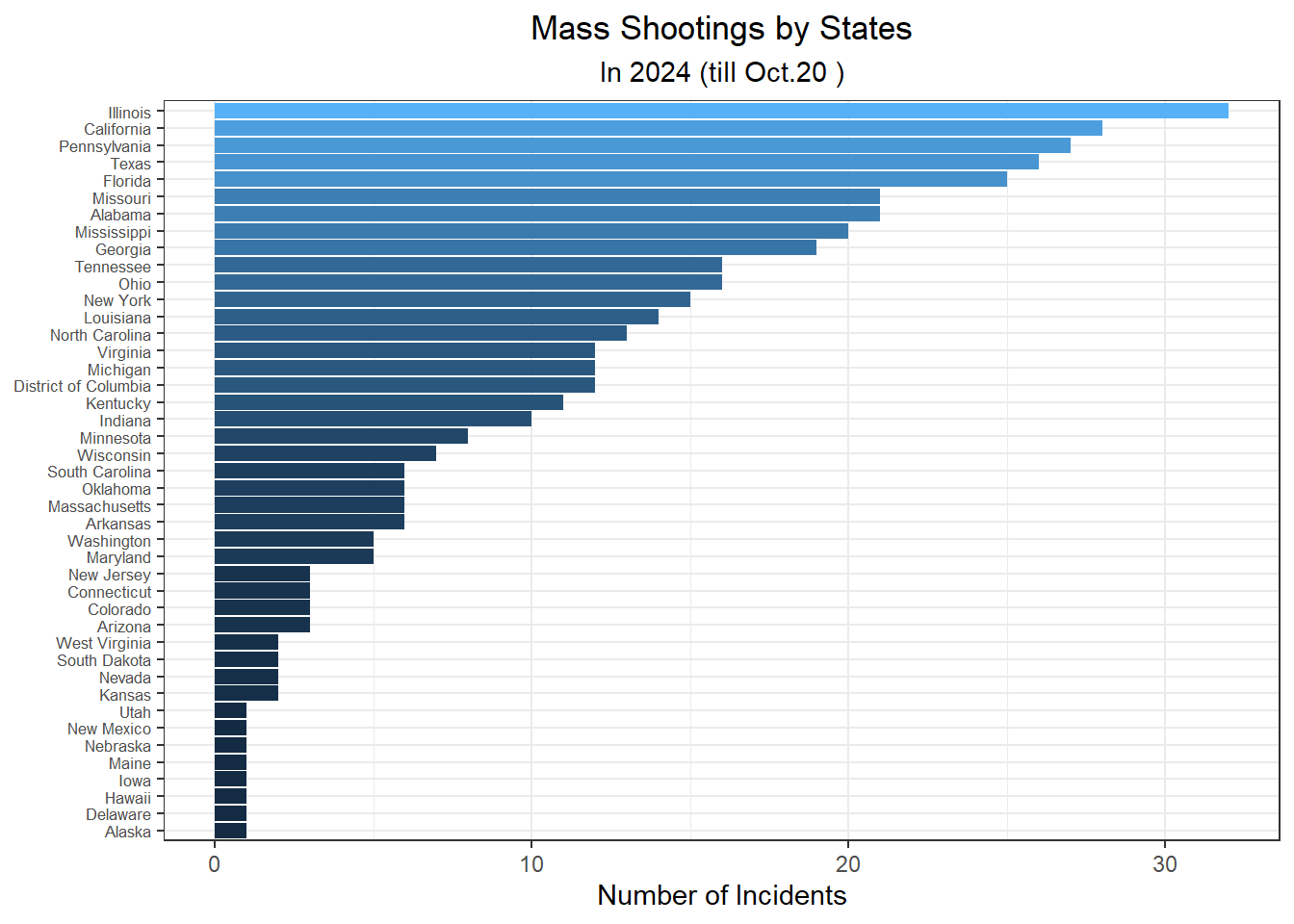
Q2. Regional patterns of mass shootings
What’s the total number of mass shootings by states?
df_time |>select(id,date,state, location, casualty)|>group_by(state)|>summarise(occurence =n())|>arrange(desc(occurence))|>ggplot(aes(x =fct_reorder(state,occurence), y = occurence, fill = occurence))+geom_col()+coord_flip()+labs(title ="Mass Shootings by States",subtitle ="In 2024 (till Oct.20 )",x =NULL,y="Number of Incidents")+theme_bw()+theme(legend.position ="none")+theme(plot.title =element_text(hjust =0.5),plot.subtitle =element_text(hjust =0.5))+theme(axis.text.y =element_text(size =6.5))
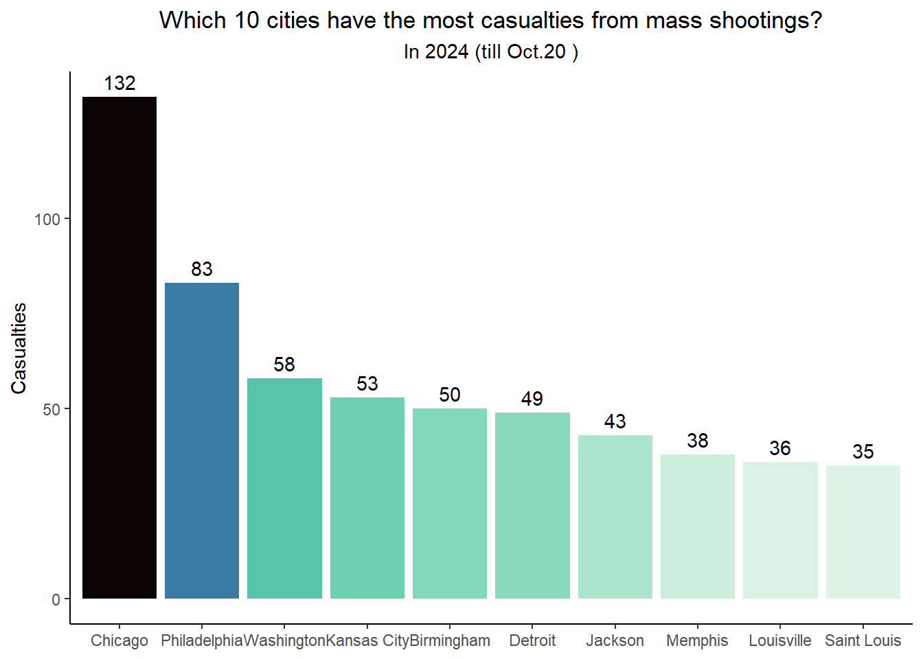
Q3. (1)What’s the total casualties (defined as individuals injured or killed) by city or county?
df_cleaned |>select(id,date,state, location, casualty)|>group_by(location)|>summarise(casualties =sum(casualty))|>top_n(10,casualties) |>ggplot(aes(x =fct_reorder(location,-casualties), y = casualties, fill = casualties))+geom_col()+scale_fill_viridis_c(option ="mako", direction =-1) +labs(title ="Which 10 cities have the most casualties from mass shootings?",subtitle ="In 2024 (till Oct.20 )",x =NULL,y="Casualties")+geom_text(aes(label = casualties), vjust =-0.5) +theme_classic()+theme(plot.title =element_text(hjust =0.5),plot.subtitle =element_text(hjust =0.5))+theme(legend.position ="none")
# A tibble: 2 × 15
       id date        state location address fatality injuries s_deceased s_hurt
    <dbl> <chr>       <chr> <chr>    <chr>      <dbl>    <dbl>      <dbl>  <dbl>
1 2928467 June 2, 20… Ohio  Akron    Kelly …        1       28          0      0
2 2808531 January 21… Illi… Joliet   200 bl…        8        1          1      0
# ℹ 6 more variables: s_detained <dbl>, operations <lgl>, lat <dbl>,
#   long <dbl>, coor <chr>, casualty <dbl>
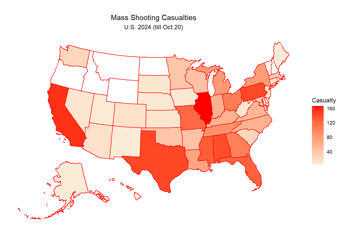
Q3. (2)What’s the total casualties by states?
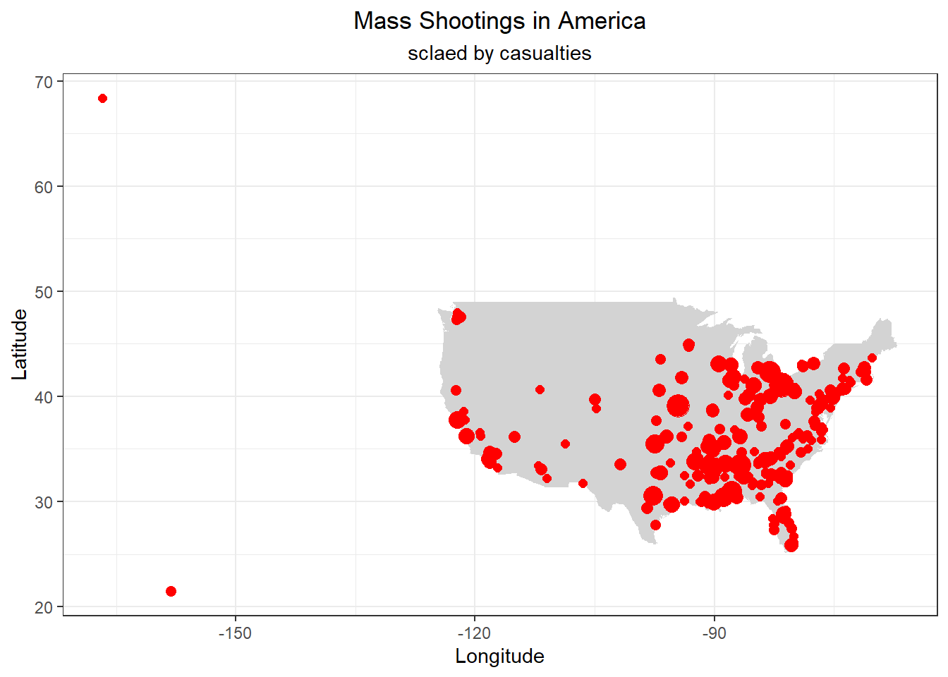
Casualties by detailed locations–scatters on map
df_cleaned <- df_cleaned |>mutate(size_num = casualty/4) # to make the point a map standardized, use 4 as division because the definition of mass shootings requires 4 or more victims
usa_map <-map_data("state")ggplot() +geom_polygon(data = usa_map, aes(x = long, y = lat, group = group), fill ="lightgrey") +geom_point(data = df_cleaned, aes(x = long, y = lat, size = size_num), color ="red") +labs(title ="Mass Shootings in America", subtitle ="sclaed by casualties",x ="Longitude",y ="Latitude") +theme_bw()+theme(legend.position ="none")+theme(plot.title =element_text(hjust =0.5),plot.subtitle =element_text(hjust =0.5))
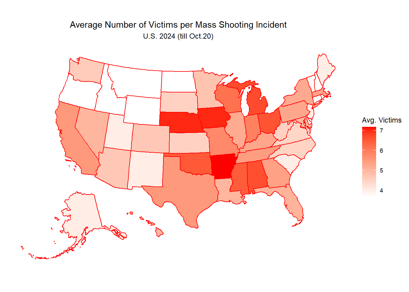
Casualties by states & Average victim numbers by incidents per state
Analysis
state_casualties <- df_cleaned |>group_by(state) |>summarize(total_casualties =sum(casualty),total_occurence =n()) |>mutate(victimization_rate = total_casualties/total_occurence) #victimization rate here means average victim numbers per incidentprint(state_casualties)
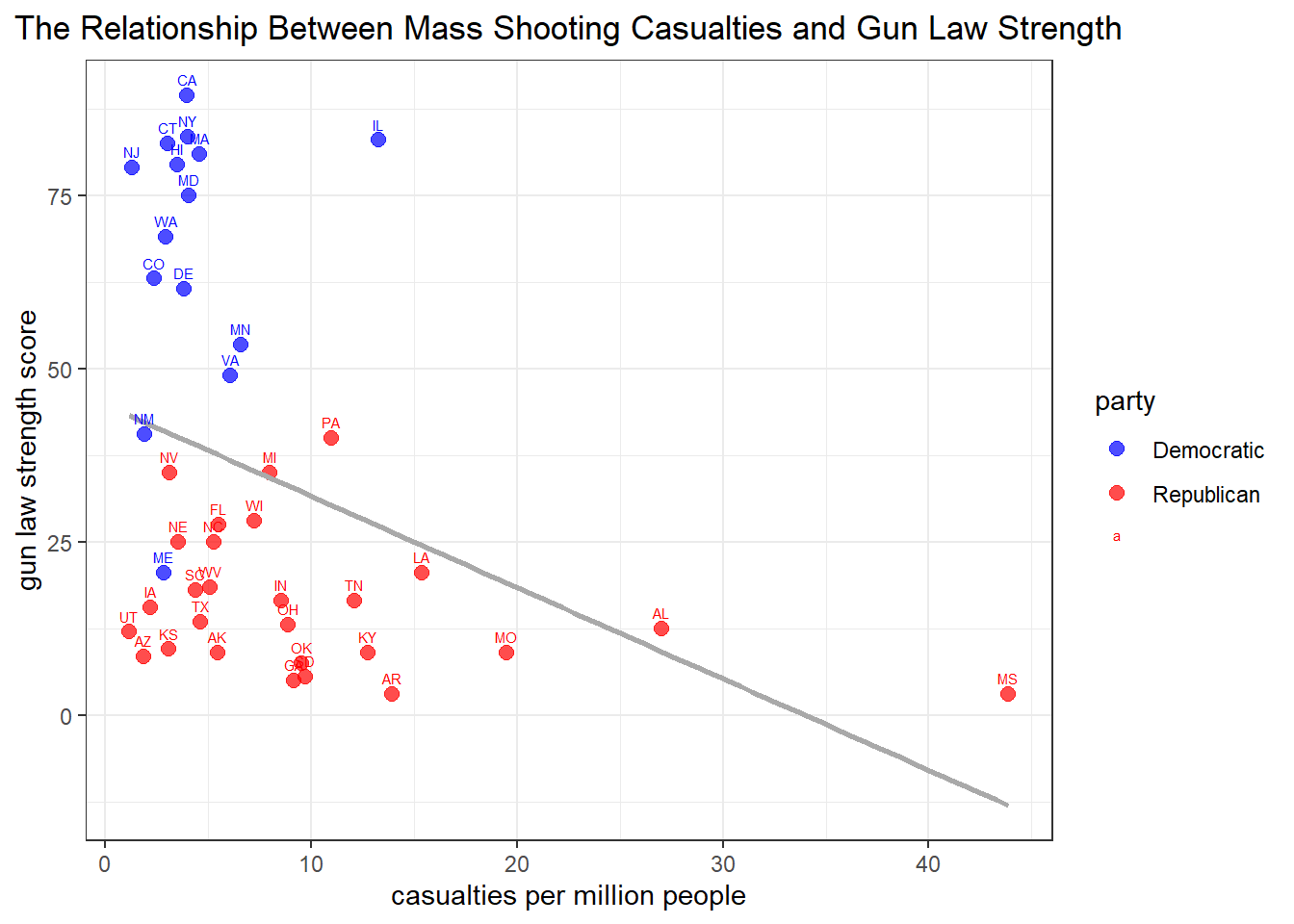
law_shootings <- state_casualties |>left_join(df_pop, by ="state") |>left_join(df_gunlaw, by ="state")|>left_join(state_abbr, by =c("state"="state_full"))glimpse(law_shootings)
law_shootings |>mutate(cas_rate = total_casualties/population *1000000)|>#use casualties per million people to provides a standardized way to compare gun violence ratesselect(state, state_abbr, cas_rate, score)|>filter(state !="District of Columbia")|># exclude the data for Distirct of Columbia, because its population and gun law strength has not been recordedmutate(party = state_party[state]) |>ggplot(aes(x = cas_rate, y = score, color = party)) +geom_point(size =2.5, alpha =0.7) +geom_smooth(method ="lm", se =FALSE, color ="darkgrey") +geom_text(aes(label = state_abbr), vjust =-0.9, size =2) +labs(title ="The Relationship Between Mass Shooting Casualties and Gun Law Strength",x ="casualties per million people",y ="gun law strength score") +theme_bw()+scale_color_manual(values =c("blue", "red"))+theme(plot.title =element_text(hjust =0.5))